Red Wine Quality Prediction
Jiafei Li, jl5548; Gaotong Liu, gl2677; Yuchen Qi, yq2279
2020/5/16
Introduction
This final project aims to find an optimal model in order to better predict red wine quality based on physicochemical tests. The original dataset contains 1599 observations of 11 predictors from physicochemical test (including PH value, density, fixed acidity, volatile acidity, citric acid, residual sugar, chlorides, free sulfur dioxide, total sulfur dioxide, sulphates, alcohol), and 1 response variable (wine quality), describing features of the Portuguese red wine “Vinho Verde”.
Data Preparation
Missing data and Variable type
We first examined variable types and missing values of the dataset. As a result, all variables are numeric and there is no variable containing missing data. We converted the response variable “quality” to factor variable of 6 levels, and collapsed them into 2 levels (“poor”, “good”) to balance the total count of different levels. Then we cleaned the dataset, and partitioned the dataset to get training(\(\frac{2}{3}\)) and testing data(\(\frac{1}{3}\)).
df.raw = read_csv("winequality-red.csv")
df = df.raw %>%
  janitor::clean_names() %>%
  mutate(quality = factor(quality,
                             labels = c("q3","q4","q5","q6","q7","q8"))) %>%
  mutate(quality = fct_collapse(quality,
                                poor = c("q3","q4","q5"),
                                good = c("q6","q7","q8")))

set.seed(1)
rowTrain <- createDataPartition(y = df$quality,
                                p = 2/3,
                                list = FALSE)
df.train = df[rowTrain,]
x = model.matrix(quality~., df.train)[,-1]
y = df.train$quality
df.test = df[-rowTrain,]
Exploratory analysis
Correlations
11 predictors are all numerical variables. There is no strong correlation (>0.7) between the predictors in the Fig 1. However, fixed_acidicity and citric_acid, fixed_acidicity and density, fixed_acidicity and p_h, free_sulfur_dioxide and total_sulfur_dioxide do have some correaltions(0.7).
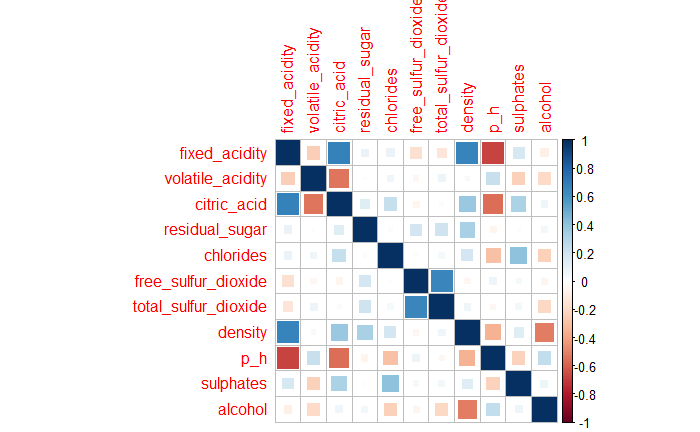 Fig 1. Correlation Matrix Plot
var.numerical = df.train %>% dplyr::select_if(is.numeric) %>% as.matrix()
var.cor = cor(var.numerical)
plot1 = cor(var.numerical) %>%
  corrplot.mixed(tl.cex = 0.7, tl.pos = "lt",
                 number.digits = 1, number.cex = .8,
                 title = "Figure 1. Correlation Matrix Plot")
which((var.cor > 0.7 & var.cor < 1), arr.ind = TRUE)
Density plot
theme1 <- transparentTheme(trans = .4)
trellis.par.set(theme1)

plot2 = featurePlot(x,
            y,
            scales = list(x=list(relation="free"),
                          y=list(relation="free")),
            plot = "density", pch = "|",
            auto.key = list(columns = 2),
             main = "Figure 2. Density plot for predictors and response(good vs poor)")
As shown in the Fig 2, most of the predictors such as ph, sulphates, free sulfur dioxide, and residual sugar have similar distributions for the good and poor quality, the alcohol predictor has slightly different distribution for good and poor quality.
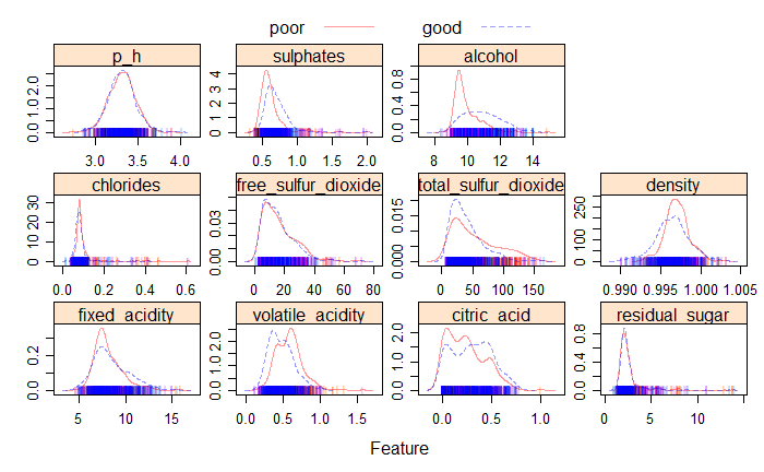 Fig 2. Density Plot
Models
All the 11 numeric predictors were included in the models. 8 classification models were used to predict the quality of the red wine (poor and good).
ctrl <- trainControl(method = "cv",
                     summaryFunction = twoClassSummary,
                     classProbs = TRUE)
Linear Discrimininant analysis (LDA)
LDA projects the feature space onto a smaller subspace while maintaining the class discriminatory information. It has the linear boundary and assumes the same covariance matrix in each class. It is quite robust to the distribution of the classification data when the sample size is small.
Quadratic Discrimininant analysis (QDA)
QDA has the quadratic boundary and assumes different covariance matrix in each class.
set.seed(1)
model.lda <- train(quality~., df,
                   subset = rowTrain,
                   method = "lda",
                   metric = "ROC",
                   trControl = ctrl)
lda.pred <- predict(model.lda, newdata = df[-rowTrain,], type = "prob")[,1]
set.seed(1)
model.qda <- train(quality~., df,
                   subset = rowTrain,
                   method = "qda",
                   metric = "ROC",
                   trControl = ctrl)
qda.pred <- predict(model.qda, newdata = df[-rowTrain,], type = "prob")[,1]
k-Nearest-Neighbor classifiers (KNN)
set.seed(1)
knn.fit <- train(quality~., df,
                   subset = rowTrain,
                   method = "knn",
                   preProcess = c("center","scale"),
                   tuneGrid = data.frame(k = seq(1,200,by=5)),
                   trControl = ctrl)

plot3 = ggplot(knn.fit)

knn.pred <- predict(knn.fit, newdata = df[-rowTrain,], type = "prob")[,1]
It predicts class label given \(x_0\) by finding k nearest points in distance to \(x_0\) and then classify \(x_0\) using majority vote among the kneighbors. The tuning parameter is k with optimal value 41 in the knn model.
Classification tree
set.seed(1)
rpart.fit <- train(quality~., df,
                   subset = rowTrain,
                   method = "rpart",
                   tuneGrid = data.frame(cp = exp(seq(-8,-5, len = 20))),
                   trControl = ctrl,
                   metric = "ROC")
plot4 = ggplot(rpart.fit, highlight = TRUE)
#rpart.plot(rpart.fit$finalModel)
rpart.pred <- predict(rpart.fit, newdata = df[-rowTrain,], type = "prob")[,1]
Tree-based method uses recursive binary splitting to segment the predictor space into simple regions according to the largest reduction of total varaince across the k classes(Gini index), then predict the class labels by the majority vote in the simple regions. Although single tree can have small bias, the variance is quite large.
CART approach is used to prune the classification tree. A large tree is grown at first and then prune it back by penalty for tree complexity(\(\alpha\) controls). The tuning parameter is cp(\(\alpha\)) with optimal value 0.003583 in the single classificaton tree model(CART).
Random Forest
rf.grid <- expand.grid(mtry = 1:6,
                       splitrule = "gini",
                       min.node.size = 1:6)
set.seed(1)
rf.fit <- train(quality~., df,
                subset = rowTrain,
                method = "ranger",
                tuneGrid = rf.grid,
                metric = "ROC",
                trControl = ctrl)

plot5 = ggplot(rf.fit, highlight = TRUE)

rf.pred <- predict(rf.fit, newdata = df[-rowTrain,], type = "prob")[,1]
Random Forest is one of the ensemble methods which uses collections of single trees to get better predictive performance(lower variance). Random Forest generate B different bootstrapped training data sets and the split in each tree is considered a random selection of m out of p(full set) predictors, then it predicts the class labels by majority vote among B trees.
The tuning parameters are mtry (m) with optimal value 1, min.node.size(minimal node size) with optimal value 1 in random forest model.(Fig 3.)
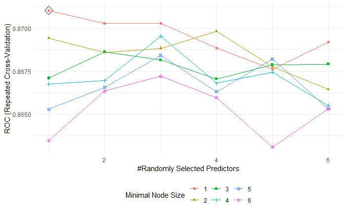 Fig 3. Random forest tuning parameters
Boositng(AdaBoost)
gbmA.grid <- expand.grid(n.trees = c(3000,4000,5000),
                        interaction.depth = 19:24,
                        shrinkage = c(0.003,0.004, 0.005),
                        n.minobsinnode = 1)
set.seed(1)
# Adaboost loss function
gbmA.fit <- train(quality~., df,
                 subset = rowTrain,
                 tuneGrid = gbmA.grid,
                 trControl = ctrl,
                 method = "gbm",
                 distribution = "adaboost",
                 metric = "ROC",
                 verbose = FALSE)

plot6 = ggplot(gbmA.fit, highlight = TRUE)

gbmA.pred <- predict(gbmA.fit, newdata = df[-rowTrain,], type = "prob")[,1]
Boosting grows tree uses information from previously grown trees. AdaBoost repeatedly fit classicication trees to weighted versions of training data and update the weights to better classify.
The tuning parameter are n.trees(the number of trees) with optimal value 5000, interaction.depth(the complexity of boosted ensemble) with optimal value 23, shrinkage(the rate of boosting learn) with optimal value 0.005, n.minobsinnode(minimal node size) with optimal value 1 in boosting model.(Fig 4.)
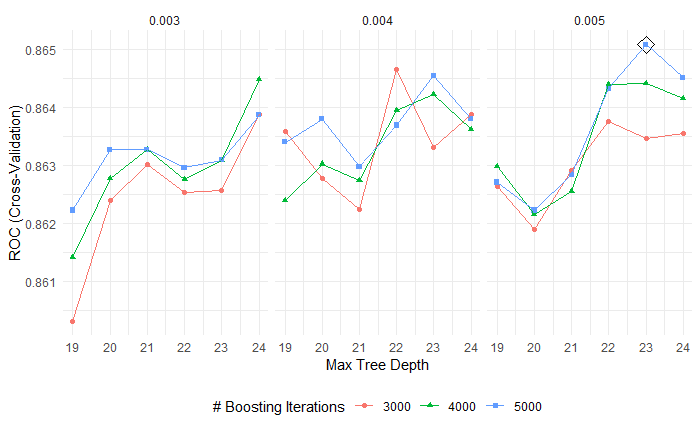 Fig 4. Boosting tuning parameters
Support Vector Machine Linear kernel(SVML)
set.seed(1)
svmlinear.fit <- train(quality~.,
                  df,
                   subset = rowTrain,
                  method = "svmLinear2",
                  preProcess = c("center", "scale"),
                  tuneGrid = data.frame(cost = exp(seq(-5, 1, len=30))),
                  trControl = ctrl)
plot7 = ggplot(svmlinear.fit, highlight = TRUE)

svml.pred <- predict(svmlinear.fit, newdata = df[-rowTrain,], type = "prob")[,1]
# train error
pred.svmlinear.train <- predict(svmlinear.fit$finalModel, data = df.train)
#confusionMatrix(data = pred.svmlinear.train,
#               reference = df$quality[rowTrain])
# test error
pred.svmlinear.test <- predict(svmlinear.fit, newdata = df.test)
#confusionMatrix(data = pred.svmlinear.test,
#               reference = df$quality[-rowTrain])
SVM finds a hyperplane to separate the class in feature space and C, as a regularization parameter, controls the margin size and shows the tolerance for observations on the wrong side. Linear kernel has linear boundary. The tuning parameter is cost(C) with optimal value 0.01019 in support vector machine with linear kernel.
Support Vector Machine Radial kernel(SVMR)
svmr.grid <- expand.grid(C = exp(seq(-4, 5,len=10)),
                         sigma = exp(seq(-8,-3,len=5)))
set.seed(1)
svmradial.fit <- train(quality~.,
                       data = df,
                       subset = rowTrain,
                       method = "svmRadial",
                       preProcess = c("center", "scale"),
                       tuneGrid = svmr.grid,
                       trControl = ctrl)
plot8 = ggplot(svmradial.fit, highlight = TRUE)
#svmradial.fit$bestTune
svmr.pred <- predict(svmradial.fit, newdata = df[-rowTrain,], type = "prob")[,1]
# train error
pred.svmradial.train <- predict(svmradial.fit, newdata = df.train)
#confusionMatrix(data = pred.svmradial.train,
#               reference = df$quality[rowTrain])
# test error
pred.svmradial.test <- predict(svmradial.fit, newdata = df.test)
#confusionMatrix(data = pred.svmradial.test,
#               reference = df$quality[-rowTrain])
Different from the linear kernel, radial kernel can construct nonlinear classification boundaries. The tuning parameters are cost(C) with optimal value 20.0855, sigma(\(\gamma\), local behavior) 0.04978 in support vector machine with radinal kernel.(Fig 5)
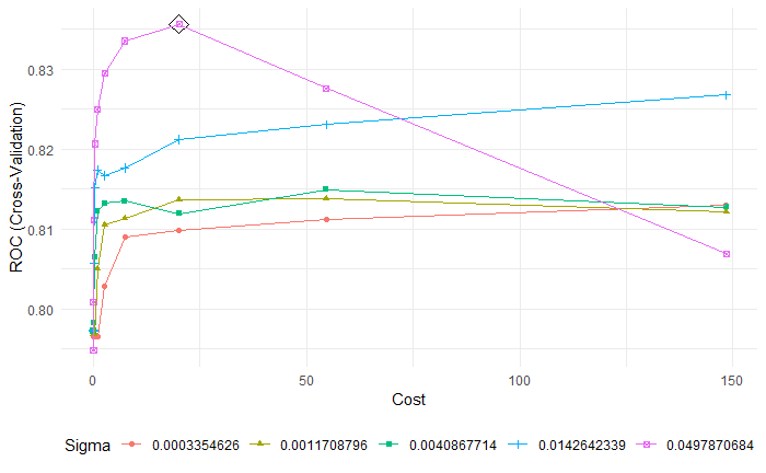 Fig 5. SVMR tuning parameters
Performance
resamp <- resamples(list(rf = rf.fit,
                         knn = knn.fit,
                         lda = model.lda,
                         qda = model.qda,
                         rpart = rpart.fit,
                         boosting = gbmA.fit,
                         svmlinear = svmlinear.fit,
                         svmradinal = svmradial.fit))
summary(resamp)
roc.lda <- roc(df$quality[-rowTrain], lda.pred)
roc.qda <- roc(df$quality[-rowTrain], qda.pred)
roc.knn <- roc(df$quality[-rowTrain], knn.pred)
roc.rf <- roc(df$quality[-rowTrain], rf.pred)
roc.rpart <- roc(df$quality[-rowTrain], rpart.pred)
roc.gbmA <- roc(df$quality[-rowTrain], gbmA.pred)
roc.svml <- roc(df$quality[-rowTrain], svml.pred)
roc.svmr <- roc(df$quality[-rowTrain], svmr.pred)
plot(roc.lda)
plot(roc.qda, add = TRUE, col = 2)
plot(roc.knn, add = TRUE, col = 3)
plot(roc.rf, add = TRUE, col = 4)
plot(roc.rpart, add = TRUE, col = 5)
plot(roc.gbmA, add = TRUE, col = 6)
plot(roc.svml, add = TRUE, col = 7)
plot(roc.svmr, add = TRUE, col = 8)
auc <- c(roc.lda$auc[1], roc.qda$auc[1], roc.knn$auc[1],
roc.rf$auc[1], roc.rpart$auc[1], roc.gbmA$auc[1],
roc.svml$auc[1], roc.svmr$auc[1])
modelNames <- c("lda","qda","knn","rf","rpart","gbmA",
"svml","svmr")
legend("bottomright", legend = paste0(modelNames, ": ", round(auc,3)),
col = 1:8, lwd = 2)From summary table of training cross validation performence, random forest has largest mean ROC. In addition, from the plot of AUC using test data, random forest has the best test performance.(Fig 6)
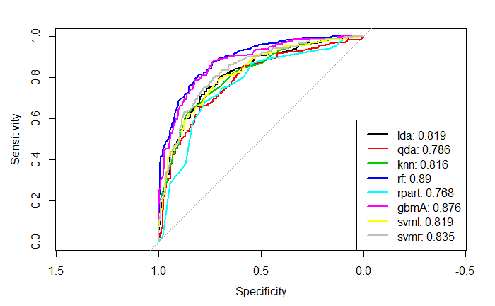 Fig 6. Test ROC
Variable importance
set.seed(1)
rf.final <- ranger(quality~., df[rowTrain,],
                        mtry = 1 ,
                        min.node.size = 1,
                        splitrule = "gini",
                        importance = "permutation",
                        scale.permutation.importance = TRUE)

plot9 = barplot(
  sort(ranger::importance(rf.final), decreasing = FALSE),
        las = 1, horiz = TRUE, cex.names = 0.6,
        col = colorRampPalette(colors = c("cyan","blue"))(11),
  main = "Figure 9: Variable importance from Random Forest")
#sort(ranger::importance(rf.final), decreasing = FALSE)
The top three variables which play important roles of predicting red wine quality are alcohol, sulphates and volatile_acidity.(Fig 7)
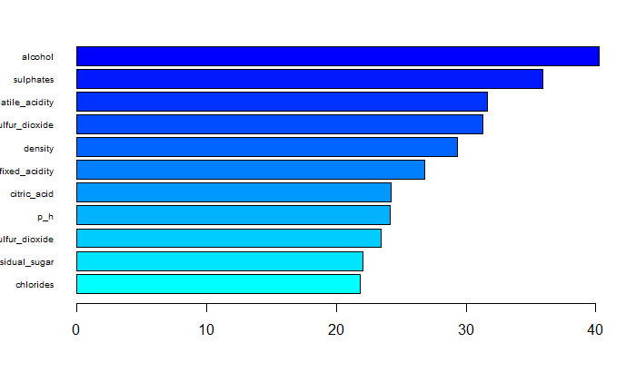 Fig 7. Variable importance
PDP
plot10 <- rf.fit %>%
  partial(pred.var = "alcohol",
          grid.resolution = 100,
          prob = TRUE) %>%
  autoplot(rug = TRUE, train = df[rowTrain,]) +
  ggtitle("Figure 10: PDP for Random forest")
The most important variable alcohol is chosen to investigate the typical influence on red wine quality across all observations. From the partial dependence plot, the higher the alcohol, the lower the quality after averaging all the effects of other predictors.
ICE
ice1.rf <- rf.fit %>%
  partial(pred.var = "alcohol",
          grid.resolution = 100,
          ice = TRUE,
          prob = TRUE) %>%
  autoplot(train = df[rowTrain,], alpha = .1) +
  ggtitle("Figure 11: ICE:Random forest, non-centered")

ice2.rf <- rf.fit %>%
  partial(pred.var = "alcohol",
          grid.resolution = 100,
          ice = TRUE,
          prob = TRUE) %>%
  autoplot(train = df[rowTrain,], alpha = .1,
           center = TRUE) +
  ggtitle("ICE:Random forest, centered")

plot11 = grid.arrange(ice1.rf, ice2.rf,
             nrow = 1, ncol = 2)
From the individual conditional expectations plot, the higher the alcohol, the lower the quality after ignoring the effects of other predictors. ICE and PDP plots are quite similar, so the alcohol is independent of other predictors.(Fig 8)
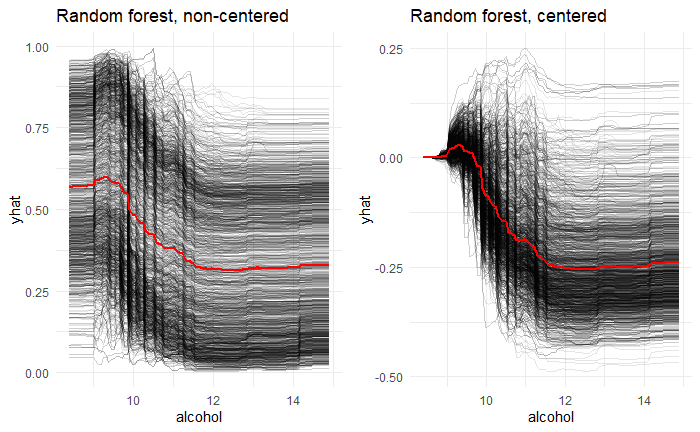 Fig 8. Individual Conditional Expectations plots
Explain prediction
new_obs <- df[-rowTrain,-12][1:2,]
explainer.rf <- lime(df[rowTrain,-12], rf.fit)
explanation.rf <- explain(new_obs, explainer.rf,
                          n_features = 3,
                          labels = "good")
plot12 = plot_features(explanation.rf)
After fitting a simple model around a single observation that mimic how th global model behaves at that locality. The prediction of two new observation can be explained by three features.
The first new observation is labeled as good quality with probability 0.21. This observation has alcohol smaller than 9.5 and this feature associates with poor quality. This observation has sulphates smaller than 0.55 and this feature associates with poor quality.This observation has chlorides smaller than 0.07 and this feature associates with good quality. (Fig 9)
The second new observation is labeled as good quality with probability 0.38. This observation has sulphates smaller than 0.55 and this feature associates with poor quality. This observation has density smaller than 0.996 and this feature associates with good quality.This observation has volatile_acidity larger than 0.64 and this feature associates with poor quality. (Fig 9)
Fig 9. Predication explainatioin(lime)
Conclusion
The performance of our models is evaluated based on ROC. The random forest model gives the best prediction performance with the ROC mean 0.8797 based on training data. Thus, for the red wine quality, we may choose random forest to predict whether it is poor or good. The test classification error rate is 0.1932 based on the confusion matrix below.
We expect that predictors having different distributions in the good and poor quality groups are important predictors, and among those predictors alcohol, total_sulfur_dioxide, volatile_acidity do play important roles of predicting red wine quality. As for the model, it is expected that the boosting model will perform best, and the lack of sufficient parameter tuning may account for the choice of random forest instead. We tried different tuning grids, and to find the best tuning parameters we need to expand the tuning grid, but it exceeds our computer capacity. Alternatively, random forest may be the optimal solution for this dataset.
rf.pred <- predict(rf.fit, newdata = df[-rowTrain,])
#confusionMatrix(data = rf.pred,
#                reference = df$quality[-rowTrain],
#                positive = "good")